How We Built Production Vector Search Inside an Analytical Database: 900 QPS at 97% Recall

Apache Doris 4.1 adds native vector search: IVF and disk-tiered SPANN indexes, PQ quantization, and hybrid BM25+vector queries planned in a single SQL.

Once LLM applications hit production, ANN vector search stops being exotic and joins the normal data plane next to filters, joins, and aggregates. The architectural question is where it should live — and what it costs to put it there.

TL;DR

• Apache Doris 4.1 ships native ANN vector indexes inside an OLAP engine: HNSW (since 4.0), and now IVF and IVF_ON_DISK (a SPANN-style disk-tiered design) for million- to billion-scale workloads.
• On a 16-core, 64 GB box against 1M × 768-dim vectors, the engine reaches 900 QPS at 97% recall on the VectorDBBench small-scale benchmark.
• INT8, INT4, and PQ quantization stack on top of IVF_ON_DISK, compressing each 768-dim vector from 3072 B to 64 B (~48×).
• Ann Index Only Scan skips the raw vector column when the query does not need it back, delivering roughly 4× end-to-end speedup.
• Structured filters, BM25 full-text search, and vector search compose inside a single SQL statement: the optimizer picks pre- vs. post-filter, and RRF fuses multi-channel recall without normalizing scores.
• Best fit when the pipeline already runs on Doris and queries mix vector with filters or text. For pure-vector workloads with extreme p99 or specialized hardware needs, dedicated vector databases still win.

1. Where Vector Search Should Live

Semantic search, RAG, recommendations, multimodal retrieval — all of them need approximate nearest neighbor (ANN) search over high-dimensional vectors. The same “where should the index live” question is being worked through one layer down at the file-format level too: see How Hard Is It to Add an Index to an Open Format for the Apache Iceberg side. This post sticks with the engine layer.

There are roughly three answers in use today.

A dedicated vector database (Milvus, Qdrant, Pinecone) is built around ANN from the ground up and tuned for pure vector workloads. The cost is that it sits next to your existing data stack as a separate system, and the application has to handle consistency, joint queries, and operations across both.

A relational extension (pgvector, MySQL HeatWave Vector) sits inside your transactional database and is cheap to roll out. The limitation is that the underlying storage and index structures were never designed for large vector workloads, so scale and concurrency hit a ceiling fairly quickly.

Native support inside an analytical database (Elasticsearch dense_vector, ClickHouse ANN, Apache Doris vector indexes) reuses the columnar storage, distributed execution, and vectorized query engine that the analytical engine already provides. That makes it a natural fit for hybrid queries that mix structured filters with vector search. The engineering challenge is integrating ANN deeply enough with an OLAP engine that the result is more than a checkbox feature.

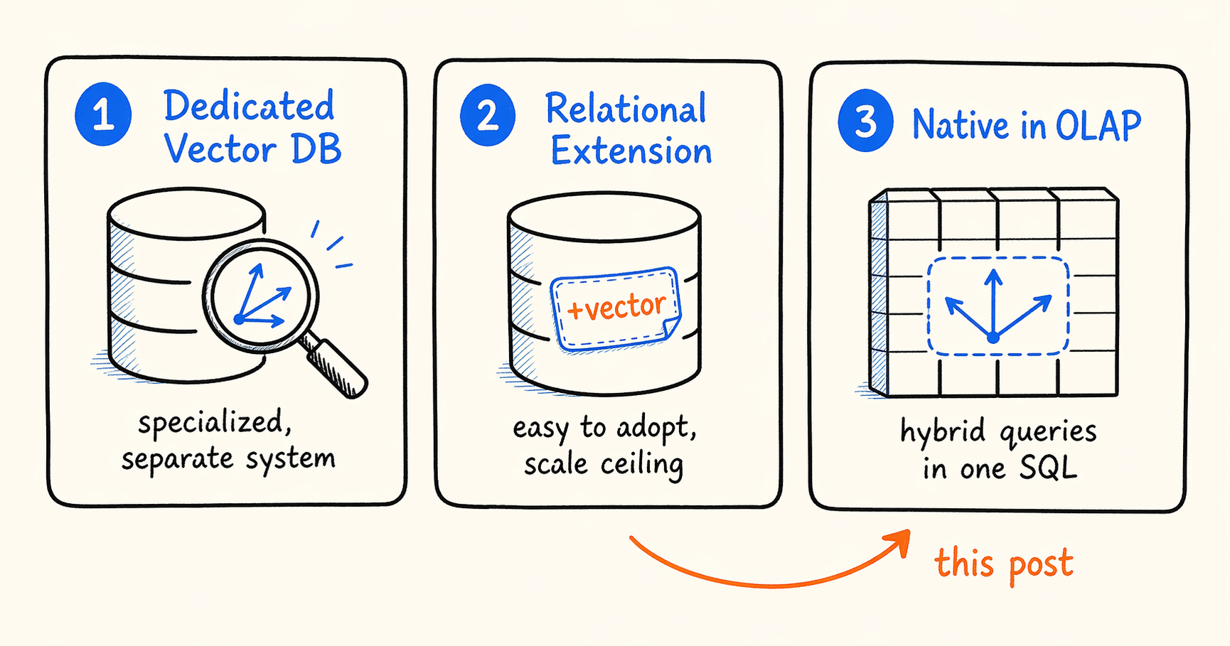
None of the three is universally better. They fit different workloads. This post focuses on the third path, and on what it took for us to make it production-grade in Apache Doris 4.1. Concretely, four questions had to be answered:

1. As vector counts grow from millions to billions, how do you control memory cost?
2. Can query performance meet online SLAs?
3. Can hybrid queries (vector search combined with structured filters or text search) run efficiently in a single SQL statement?
4. Is recall good enough for the workload?

The sections below take each of these in turn, walk through the common industry approaches, and use what we shipped in Doris 4.1 as the worked example. The headline numbers are in the TL;DR above; the sections below show the work behind them.

---

2. Memory Cost as the Dataset Grows

Memory consumption in vector search does not come only from the vectors.

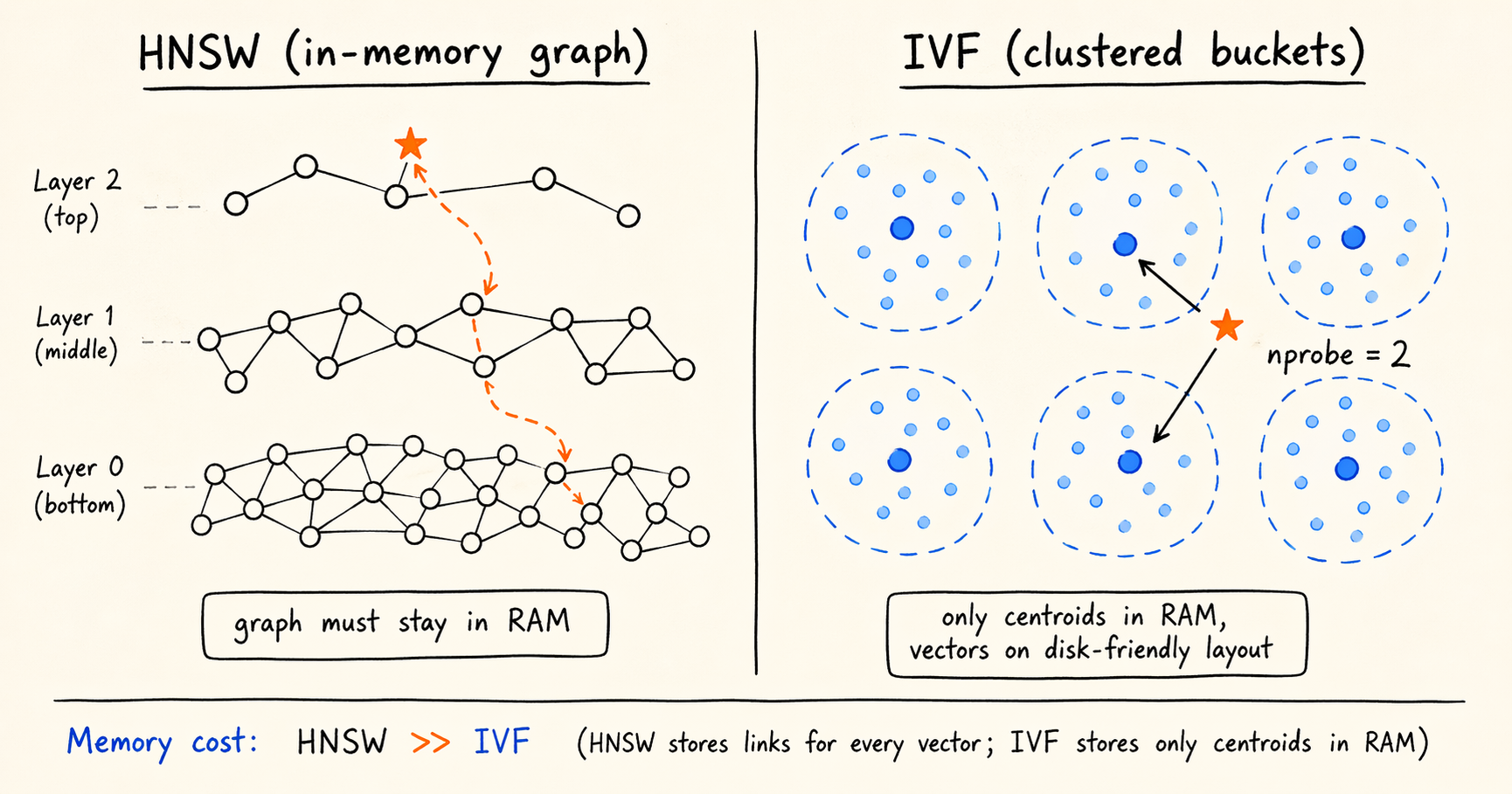
Take 1 million 768-dimensional float32 vectors. The raw data is 1,000,000 × 768 × 4 ≈ 3 GB. On top of that, the ANN index has its own memory footprint. The representative algorithm here is HNSW (Hierarchical Navigable Small World), a hierarchical navigation graph that gives high recall at logarithmic query complexity and is the usual choice at small to medium scale. The catch is that HNSW’s graph has to stay resident in memory. With common parameters (M=16, efConstruction=200), the index roughly doubles the raw data footprint. Scale that to a billion vectors and you are looking at close to 1 TB of memory. The system can still run; the deployment cost is simply not something most teams will sign off on.

IVF: A Coarser Structure for a Smaller Memory Budget

Once HNSW hits the memory ceiling, the standard alternative is IVF (Inverted File). The mechanic has two steps:

1. Build phase. Run k-means over all vectors to produce nlist centroids. Assign each vector to its nearest centroid (its bucket).
2. Query phase. Compare the query vector against the nlist centroids, take the nprobe closest buckets, and compute exact distances only inside those buckets.

Recall drops slightly, because the true top-K can land in a bucket that was not selected. In return, queries get an order-of-magnitude speedup and the index footprint shrinks substantially. IVF does not need a resident graph: memory only has to hold the centroids and the bucket-to-ID mapping, while the vectors themselves can live on disk. That last property is what makes the storage tiering in the next section possible.

The IVF Index in Doris 4.1

We added HNSW indexes in Doris 4.0, and added an IVF type in 4.1 for larger workloads. The DDL:

CREATE TABLE vecs (
  id BIGINT NOT NULL,
  embedding ARRAY<FLOAT> NOT NULL,
  INDEX idx_emb (embedding) USING ANN PROPERTIES (
    "index_type" = "ivf",
    "metric_type" = "l2_distance",
    "dim" = "768",
    "nlist" = "1024"
  )
) ENGINE=OLAP
DUPLICATE KEY(id)
DISTRIBUTED BY HASH(id) BUCKETS 8
PROPERTIES ("replication_num" = "1");

nprobe is a session-level parameter, so a single IVF index can move along the recall/latency curve at runtime without being rebuilt for different targets.

Sizing and Parameter Notes

IVF works best from tens of millions up to roughly a billion vectors. Below 100,000 vectors, or for workloads that are extremely recall-sensitive, HNSW is still the better fit. We did not retire HNSW in 4.1; IVF is a second path for the larger end.

For nlist, a reasonable starting range is √N to 4√N, but the optimum depends on the data distribution, so it is worth validating on a sample first. For nprobe, 1% to 5% of the bucket count is a common starting point; tune upward until the recall target is hit.

What IVF saves is the index structure footprint, not the vector data. The data still grows linearly with the dataset. Cutting that further requires moving storage off memory entirely, which is the next section.

---

3. Storage Tiering at Billion Scale

Using the same arithmetic, 1 billion 768-dimensional vectors occupy roughly 3 TB. Provisioning a 3 TB memory instance just for vector search is uneconomical in almost every scenario. Every vector system runs into this constraint sooner or later.

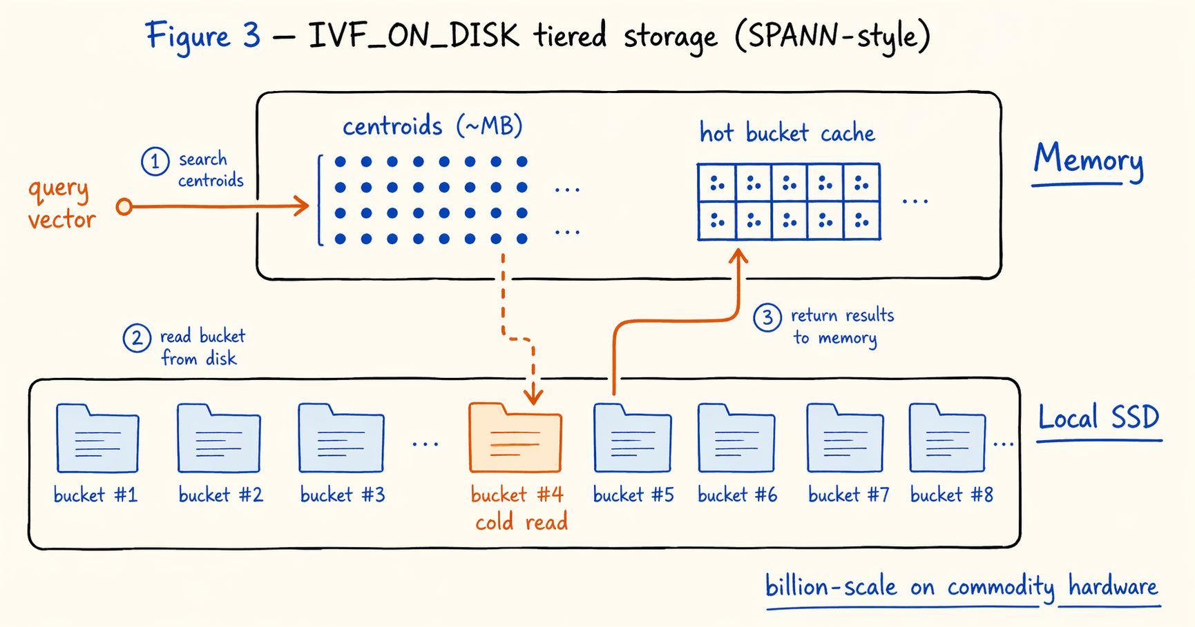
The standard answer is storage tiering: push vector data to disk and keep only the navigation structures and hot data in memory. Microsoft’s DiskANN (NeurIPS 2019) and SPANN (NeurIPS 2021) are the most cited work in this direction. SPANN in particular showed that an IVF-based tiered design holds up at billion scale.

SPANN, and the IVF_ON_DISK Implementation

Our IVF_ON_DISK index in 4.1 follows SPANN’s general layout. Centroids stay in memory: they are megabytes, negligible against the rest of the budget. Bucket data lives on disk, with each bucket’s posting list laid out sequentially in a local file and read on demand. The query path uses a cache for hot buckets; cold buckets are read through the file system.

With this layout, billion-scale search runs on commodity hardware. Memory only has to cover centroids and the working set of hot buckets; everything else stays on local disk. The DDL is essentially identical to plain IVF, with a different index_type:

CREATE TABLE vecs_large (
  id BIGINT NOT NULL,
  embedding ARRAY<FLOAT> NOT NULL,
  INDEX idx_emb (embedding) USING ANN PROPERTIES (
    "index_type" = "ivf_on_disk",
    "metric_type" = "l2_distance",
    "dim" = "768",
    "nlist" = "4096"
  )
) ENGINE=OLAP
DUPLICATE KEY(id)
DISTRIBUTED BY HASH(id) BUCKETS 32
PROPERTIES ("replication_num" = "1");

nlist usually grows with the dataset, to keep the average bucket size in check.

Performance Characteristics of the Disk Index

Intuitively, a “disk index” sounds far slower than an in-memory one. With a reasonable cache configuration, IVF_ON_DISK’s QPS is in fact close to in-memory IVF. The reason lies in the I/O pattern: neighboring queries tend to hit the same clusters, so cache hit rates are much higher than for a full scan workload. That is also why storage tiering keeps showing up as the workable answer across vector systems.

Factors to Evaluate Before Adopting It

Cold-start latency. The first access to a cold bucket pays a disk I/O, and p99 can be 5x to 10x the hot baseline. Services that take traffic immediately after startup need a warmup step in the deployment pipeline; latency-sensitive workloads need to load-test the cold case explicitly.

Disk type. The design assumes SSDs. Mechanical disks cannot handle the random read pattern.

Cache ratio. Too high and the configuration converges back to in-memory, which negates the tiering benefit. Too low and hit rate drops, which causes latency jitter. The official documentation gives starting points by data scale, but production deployments should still load-test against real query distributions.

Build cost. The disk layout adds steps to index construction, raising build time roughly 30% to 50% over in-memory IVF, depending on disk throughput and dataset size.

Storage tiering takes layout-level cost optimization about as far as it goes. The next axis is the size of each vector itself.

---

4. Compressing the Vectors Themselves

Storage tiering trades disk capacity for memory budget. It reduces total resource use but does not change how big each vector is. Further compression has to come from reducing the precision of the vector representation. That is what vector quantization does.

Quantization methods generally fall into two groups.

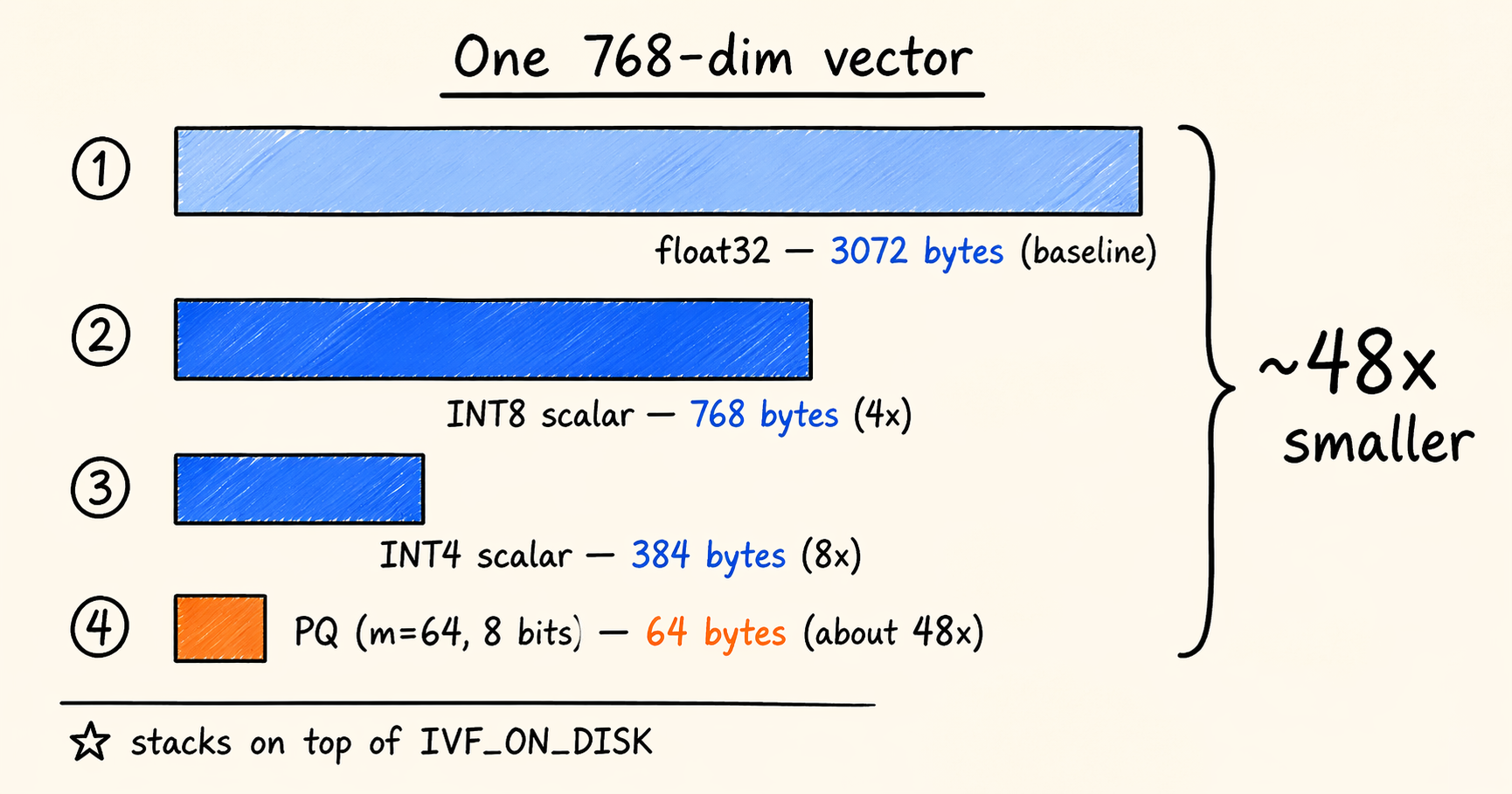
Scalar quantization compresses each dimension independently, mapping float32 (32 bits) to a narrower integer. INT8 (4x compression) and INT4 (8x compression) are the common configurations. The implementation is simple, the build is cheap, and the approximation error is predictable.

Product Quantization (PQ) splits the high-dimensional vector into m sub-vectors, runs k-means on each to produce a codebook, and represents the original vector with codeword indices. Compression ratios are higher and tunable, which is why PQ shows up in most large-scale vector search systems.

Doris 4.1 supports all three (INT8, INT4, PQ) and lets them stack on top of IVF_ON_DISK, so quantization sits on top of disk tiering. A PQ example:

CREATE TABLE vecs_pq (
  id BIGINT NOT NULL,
  embedding ARRAY<FLOAT> NOT NULL,
  INDEX idx_emb (embedding) USING ANN PROPERTIES (
    "index_type" = "ivf_on_disk",
    "metric_type" = "l2_distance",
    "dim" = "768",
    "nlist" = "4096",
    "quantizer" = "pq",
    "pq_m" = "64",
    "pq_nbits" = "8"
  )
) ENGINE=OLAP
DUPLICATE KEY(id)
DISTRIBUTED BY HASH(id) BUCKETS 32
PROPERTIES ("replication_num" = "1");

pq_m is the number of sub-vectors (768 dimensions split into 64 segments of 12 dimensions each). pq_nbits is the codeword width (8 bits gives 256 centroids per segment). Together these parameters take each vector from 3072 bytes to 64 bytes, about a 48x reduction.

Factors to Evaluate Before Adopting It

Accuracy loss. Depending on data distribution and parameters, 4x to 8x compression typically costs 1% to 3% in recall. PQ loses more at higher compression ratios. The recall floor for the workload is the primary input to the choice of method.

Build cost. Quantized indexes need extra clustering and encoding steps, so build time is higher than for plain IVF.

Combination strategy. INT8 is a reasonable starting point for recall-sensitive workloads that are only moderately cost-sensitive. PQ fits cost-sensitive workloads that can absorb some accuracy loss. A staged path also works: validate that INT8 meets the recall bar first, then decide whether PQ is worth a second migration.

Once the vectors are compressed, the remaining axis is the latency of the query path itself.

---

5. Cutting Query Latency Further

An ANN query has three main cost centers: selecting candidate buckets, computing distances to candidate vectors, and ranking the top-K. Distance computation needs the candidate vector data, which in a columnar engine means random reads against the raw vector column. With a typical nprobe × average vectors per bucket in the tens of thousands, those column reads dominate latency.

If a query only needs the top-K primary keys and distances and does not need the raw vectors back, the read against the vector column can in principle be skipped. The same idea shows up in relational databases as index-only scan: if the index already covers every column the query needs, the base table read is unnecessary.

Ann Index Only Scan

That is the idea behind the Ann Index Only Scan we shipped in 4.1. Distance computation uses the vector data already held in the index (or its quantized form) directly, without going back to the original vector column. The optimization composes with quantization and IVF_ON_DISK.

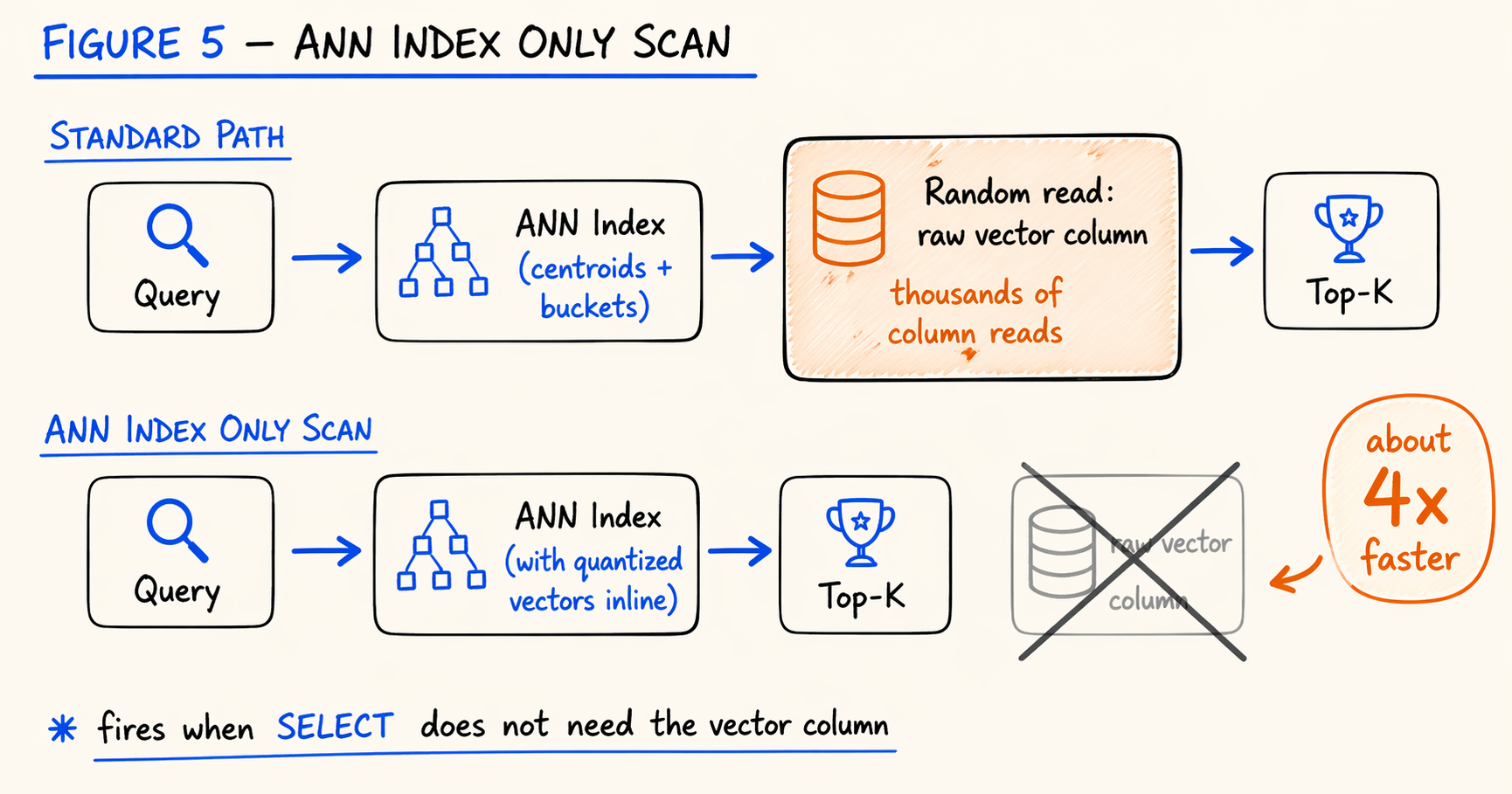
In our official baseline (16-core 64 GB single machine, 1 million 768-dimensional vectors, top-10 nearest neighbor queries), this optimization delivers about a 4x end-to-end gain, taking the final number to 900 QPS at 97% recall.

Factors to Evaluate Before Adopting It

Trigger conditions. The optimization only fires when the query result does not need the original vector column. Queries like SELECT embedding, ... fall back to the standard path.

Use with quantization. When Index Only Scan reads quantized vectors, the distances are approximate. Accuracy-sensitive workloads can enable reranking: filter the candidate set with quantized distances, then compute the final top-K against the original vectors. Accuracy returns at the cost of a small extra latency.

Limits of the gain. The 4x figure is for one specific test configuration. Different dataset sizes, dimensions, hardware, and query patterns will produce different numbers. Production deployments should load-test against real queries.

All of these optimizations target vector search in isolation. A separate question is how vector search combines with other retrieval channels.

---

6. Hybrid Queries: Structured Filters and Multi-Source Fusion

Pure vector search is rare in real workloads. Most production scenarios layer additional retrieval dimensions on top of vector similarity. Two patterns dominate.

Joint filtering with structured fields. Vector similarity combined with boolean or range filters on category, price, time, permissions, and so on. Typical examples are similar-product recommendations in e-commerce, related-content recommendations on content platforms, and tenant or time slicing in RAG.

Fusion across recall channels. Vector recall combined with text search (BM25), behavior-based recall, rule-based recall, and others, ranked together. Typical examples are hybrid search in search engines and retrieval quality improvements in RAG pipelines.

The engineering challenges they raise are different, and we will treat them separately.

Structured Filter Combined With Vector Search

Dedicated vector databases generally offer two paths for this kind of query, each with its own cost.

Post-filter (vector first, filter after) lets the vector index return top-K, then applies the structured filter at the application or gateway layer. The problem is that filtering shrinks the result set. If the filter pass rate is 30%, the actual return is only K × 30% rows, which leaves recall short.

Pre-filter (filter first, vector after) narrows the candidate set with structured conditions and then computes vector distances over that subset. The problem is that the subset has lost its IVF or HNSW structure and now requires a brute-force scan, with latency growing linearly in the candidate set size.

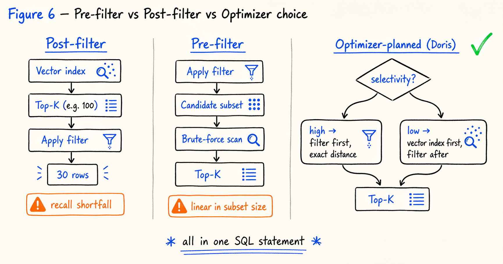
This is where native vector indexing inside an analytical database earns its keep. The query optimizer can choose between pre-filter and post-filter based on predicate selectivity, index availability, and cost estimates. The choice is not something the application has to make in advance.

A products table holds product metadata and visual embeddings. The query: within the “sneakers” category, find the 20 in-stock products priced between 50 and 200 yuan that are visually most similar to a reference product.

SELECT
  id,
  name,
  price,
  l2_distance(embedding, [0.12, 0.08, ..., 0.31]) AS distance
FROM products
WHERE category = 'sneakers'
  AND in_stock = TRUE
  AND price BETWEEN 50 AND 200
ORDER BY l2_distance(embedding, [0.12, 0.08, ..., 0.31])
LIMIT 20;

At execution time, the optimizer picks a path based on selectivity. When the structured filter is highly selective (the candidate set is much smaller than nprobe × average bucket size), the filter runs first and exact distances are computed over the subset. When the filter is weakly selective, the vector index runs first and the filter is applied to its result.

The whole flow lives in a single SQL statement. There is no static pre/post-filter choice for the application to make, and no cross-system data sync to manage.

Fusion Ranking Across Multiple Recall Channels

Multi-channel fusion presents a different problem. The question is not where filter logic should sit, but how to combine scores measured in different units. The canonical case is fusing text search with vector search. When a user types a query, the system should surface keyword hits (inverted index plus BM25) and also return results that are semantically related but may not contain the keyword (vector index plus distance). The two channels produce scores on entirely different scales: BM25 and L2 distance have no comparable basis for weighted combination.

The common answer is Reciprocal Rank Fusion (RRF) (Cormack, Clarke, Buettcher, SIGIR 2009). Instead of normalizing and weighting raw scores, RRF uses only the rank each result holds in each channel and sums the reciprocals 1 / (k + rank) to produce a final score. There is no score normalization, the method is robust to outliers, and adding a new recall source slots in cleanly. RRF shows up in most recent hybrid search deployments for those reasons.

Implementing fusion inside an analytical database means the entire pipeline fits in a single SQL statement. The example below uses RRF to fuse BM25 text search with ANN vector search on a HackerNews dataset:

WITH
  text_raw AS (
    SELECT id, score() AS bm25
    FROM hackernews
    WHERE (`text` MATCH_PHRASE 'hybrid search'
           OR `title` MATCH_PHRASE 'hybrid search')
      AND dead = 0 AND deleted = 0
    ORDER BY score() DESC
    LIMIT 1000
  ),
  vec_raw AS (
    SELECT id, l2_distance_approximate(`vector`, [0.12, 0.08, ...]) AS dist
    FROM hackernews
    ORDER BY dist ASC
    LIMIT 1000
  ),
  text_rank AS (
    SELECT id, ROW_NUMBER() OVER (ORDER BY bm25 DESC) AS r_text FROM text_raw
  ),
  vec_rank AS (
    SELECT id, ROW_NUMBER() OVER (ORDER BY dist ASC) AS r_vec FROM vec_raw
  ),
  fused AS (
    SELECT id, SUM(1.0 / (60 + rank)) AS rrf_score
    FROM (
      SELECT id, r_text AS rank FROM text_rank
      UNION ALL
      SELECT id, r_vec  AS rank FROM vec_rank
    ) t
    GROUP BY id
    ORDER BY rrf_score DESC
    LIMIT 20
  )
SELECT f.id, h.title, h.text, f.rrf_score
FROM fused f
JOIN hackernews h ON h.id = f.id
ORDER BY f.rrf_score DESC;

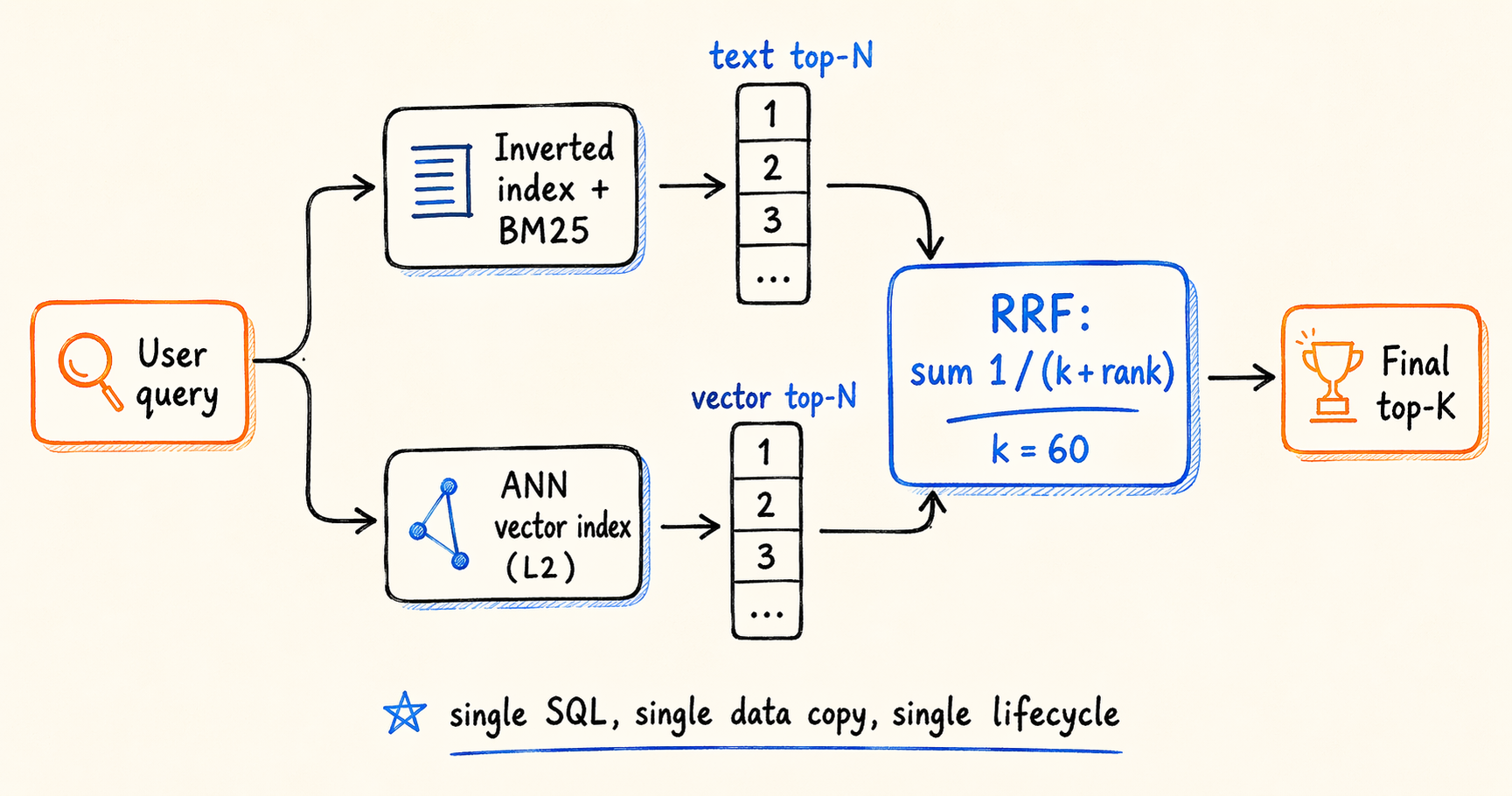
The execution path is four steps. The inverted index and the ANN index run BM25 and L2 distance recall in parallel, each taking its own top-N. The two result sets are then ranked locally based on their raw scores. For each candidate, the per-channel rank contribution 1 / (k + rank) is summed to produce the final score. Only the final top-K reads back to the base table for display fields, which avoids scanning wide columns in intermediate steps.

The value of pulling fusion into the SQL layer is not algorithmic. RRF can be implemented anywhere. The practical benefit is that both retrieval channels share the same data, the same transactional visibility, and the same lifecycle management. Extending to a third channel (weighted by category, time, or user profile) is also straightforward when the workload calls for it.

Factors to Evaluate Before Adopting It

Optimizer maturity. Selectivity estimation for complex predicates (multi-column function expressions, subqueries, filters inside joins) is not always accurate. We recommend verifying the execution plan with EXPLAIN before shipping.

Indexes on the structured columns. Inverted indexes, prefix indexes, or partition pruning on the filter columns significantly affect which path the optimizer picks. A high-cardinality column with no index does not automatically translate strong filter selectivity into a performance win.

The rank-fusion assumption. RRF discards the magnitude of raw scores, which means a very strong signal from a high-confidence channel gets flattened. The k value (commonly 60) shapes the weight distribution at the head of the list. If signal strength matters, a reranking model on top of fusion results can recover it.

Value ceiling for pure-vector workloads. If a workload rarely involves structured filters or multi-channel fusion, the differentiation discussed in this section carries less weight in the selection decision.

With memory, storage, latency, and hybrid queries covered, the remaining question is how this kind of system compares against the rest of the field in public benchmarks.

---

7. Reading the Public Benchmarks

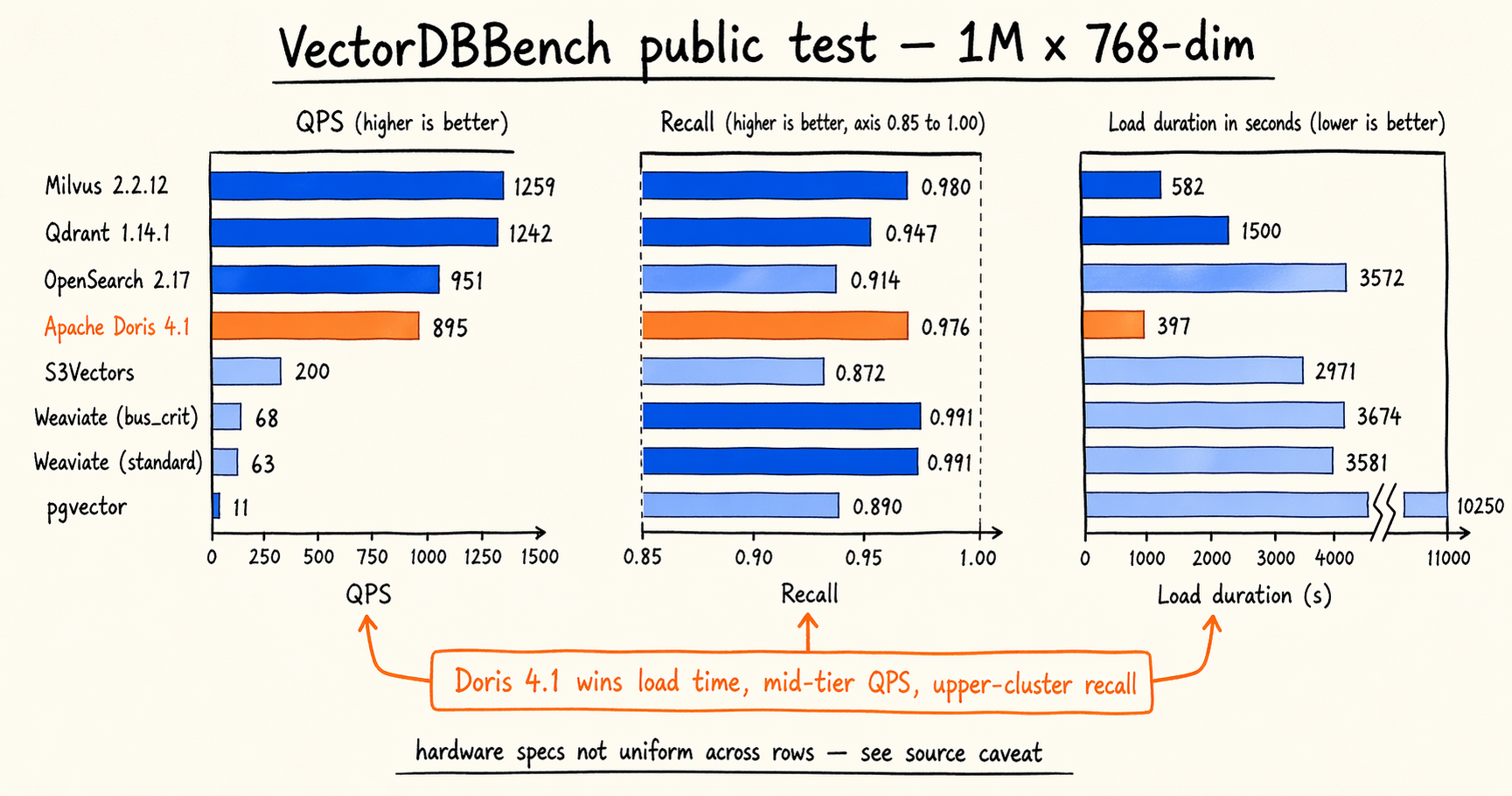
VectorDBBench’s public test data from January 2026 is a useful reference. The table below shows results for mainstream vector search systems on the 1 million × 768-dimensional dataset, sorted by QPS:

Solution (version / config)	QPS	Recall	Load duration
Milvus 2.2.12 (HNSW, 16c64g)	1,259	0.9799	581.8 s
Qdrant Cloud 1.14.1 (16c64g)	1,242	0.9474	1,500 s
OpenSearch 2.17 (16c128g)	950.6	0.9140	3,572 s
Apache Doris 4.1 (mixture, 16c64g)	895	0.9764	397 s
S3Vectors	199.5	0.8717	2,971 s
Weaviate Cloud (bus_crit)	67.91	0.9909	3,674 s
Weaviate Cloud (standard)	63.14	0.9910	3,581 s
pgvector (2c8g)	10.63	0.8898	10,250 s

Source: VectorDBBench public test (1M dataset, 768 dimensions). mixture is the hybrid index configuration Doris uses under this benchmark. One caveat worth flagging: hardware specs are not uniform across rows. OpenSearch runs on 16c128g, pgvector on 2c8g, and Weaviate Cloud and S3Vectors are managed services where the platform picks the spec. Treat row-to-row comparisons accordingly.

A look at each dimension:

Load duration (index build time). Doris 4.1 (397 s) is the fastest in this table, about 30% faster than Milvus HNSW (581.8 s) and more than an order of magnitude faster than pgvector (10,250 s). This dimension matters most for batch cold starts, index rebuilds after an embedding model change, and historical backfills. Build time translates directly into production availability and retry cost.

QPS (query throughput). Milvus and Qdrant lead the field at 1,200 plus. Doris 4.1 (895) and OpenSearch (950.6) sit in the same second tier. Weaviate Cloud and pgvector are lower, but each corresponds to either higher recall or more limited hardware.

Recall. The two Weaviate Cloud configurations (0.9910 / 0.9909) lead. Milvus, Doris, and Qdrant cluster in the second tier above 0.94. OpenSearch sits at 0.914. pgvector and S3Vectors come in below 0.9.

The data does not support a single “best” verdict. Each system lands at a specific point in the three-dimensional space of accuracy, throughput, and build cost. High QPS often comes with lower recall (Qdrant). High recall often comes with lower QPS (both Weaviate tiers). Doris 4.1’s lead on load duration paired with mid-to-upper QPS and recall is just another tradeoff combination. Benchmark numbers are useful only when the test scenario lines up with the workload. A more useful way to read the table is to map each dimension to your own priorities. Workloads with frequent index rebuilds should weight load duration heavily. Workloads with strict p99 or recall floors should run targeted load tests at their own operating point.

With those three dimensions in mind, the following rough mapping makes the selection decision more concrete:

Workload Characteristic	Preferred Solution	Reason
Data pipeline already runs on an analytical database	Native (Doris 4.1 and peers)	No dual-write or sync; hybrid queries finish in SQL
Vector search combined with structured filtering (e-commerce, RAG, recommendations)	Native	The optimizer plans across both, no static pre/post-filter choice
Pure vector workload with extreme QPS or p99 requirements	Dedicated vector database	Deeper specialization, broader operator and feature stack
Billion-plus scale, pure vector, cost-sensitive	Evaluate case by case	Both options have viable paths; pick on ecosystem fit and operational cost
Small to medium scale with strong transactional constraints	Relational extension	Transactional consistency is a hard requirement
Depends on GPU acceleration, special distance functions, or specific ANN variants	Dedicated vector database	Mature support for specialized hardware and algorithms

The “preferred solution” column is a relative call. Actual selection also depends on the team’s existing tech stack, operational capacity, and how the workload is expected to evolve. Benchmark numbers quantify the feasibility boundary of each candidate for a target scenario; they do not produce a ranking.

---

8. Fit Boundaries

Based on the previous seven sections, the native-vector-index-in-an-analytical-database path, with Apache Doris 4.1 as our reference implementation, has the following fit boundaries.

A good fit when:

• The data pipeline already runs on Doris (or is on the migration roadmap), and adding a separate system just for vector search is undesirable.
• The workload mixes vector queries with structured filters, or fuses vector and text recall channels.
• Vector scale sits between millions and billions.
• Reducing system count and operational load is an explicit goal.
• A 1% to 3% recall loss is acceptable in exchange for cost and architectural simplification.

A poor fit when:

• The workload is pure vector and depends on advanced features specific to a dedicated library (GPU acceleration, specialized distance functions, particular ANN variants).
• Scale is very large (tens of billions or more) with millisecond p99 latency as a hard constraint. This case calls for targeted load testing before a decision.
• Integrating structured data is not on the roadmap, and there is no goal to consolidate the system stack.

These boundaries are not static. As the optimizer matures and additional index types land, parts of the “poor fit” zone will move into the “good fit” zone.

---

9. Getting Started and Resources

• Apache Doris 4.1 download
• Vector index documentation